Last month in the first part of the dataviz series post I mentioned working on a Haskell version of the project.

It was a lot harder working in Haskell than working in Python - mostly because I’m unfamiliar with the language and its quirks. Installation was also a hurdle to overcome.

In this tutorial write-up I attempt to sum up important bits from the past 3 weeks and perhaps you will learn from my experience.

The code I’m referring to in this tutorial is also in this notebook.

Table of Contents

• 1. Setting up iHaskell
  • Where to get it
  • iHaskell interface
• 2. Parsing JSON data and formatting time
  • Aeson decoder
  • Designing before coding
  • Sorting and grouping
• 3. Setting up Plots with iHaskell
  • iHaskell Configs
  • Heatmap examples
  • Creating plots

1. Setting up iHaskell

Currently as of this writing the latest version of GHC is on 8+, which means that your ghc-parser needs to match. The original iHaskell repo that is called from hackage (cabal install ihaskell) and stackage (stack install ihaskell) are both outdated¹.

There’s a few extra options to install beyond the baseline iHaskell installation. Go to section 3. Setting up Plots with iHaskell to see the instructions for using iHaskell with Plots.

Where to get it

What you should do to install iHaskell on GHC8+ is use this other repo that is a fork of the original. Documented in issue #690

Read carefully for a quick second… use the macos-install.sh script to install dependencies. I missed the existence of this script the first few times I tried to install this, lordy lordy²

iHaskell interface

iHaskell, which I’m guessing stands for interactive haskell uses the jupyter notebook format, which is nice to work with while learning to code because I can slowly iterate and keep a record of what I’m learning.

If you’ve seen Jupyter, or used it before, the interface is the same. You can run code snippets or write markdown formatted text.

I really like the workflow of trying a few things and then writing notes in plain English to myself afterwards.

2. Parsing JSON data and formatting time

I had the data saved in a JSON file earlier, and read from this file. A library for working with JSON is the aeson library. I say working with because from what I understand aeson helps with parsing rather than reading files. Though parsing could arguably be a subset activity of reading… so… idk ¯\_(ツ)_/¯

Aeson decoder

Anyway, to include aeson capabilities, you need to import the package. Then you need to define the structure of the JSON field names.

{-# LANGUAGE DeriveGeneric #-}

import Data.Aeson
import Data.Aeson.Types
import Data.Time.Clock (UTCTime)
import Options.Generic

data Post = Post
  { created_time :: UTCTime
  , id           :: String
  , message      :: Maybe String
  , story        :: Maybe String
  } deriving (Show, Generic)

-- FYI: use of Generic requires importing and setting language flag above

instance FromJSON Post
instance ToJSON Post

Some thoughts about this code…

• I don’t remember why I used Generic.. (sadly) and will have to research later what Generic means.
• I was able to define the UTC timestamp strings upon parsing, which is awesome. Contrasting to Python which required an extra step of dateutil.parser.parse on the timestamp string.
• Reading the text file is a matter of using ByteString’s readFile

At this point I haven’t figured out how Bytestring, Text, String, etc types are different. Aeson uses Bytestring so that’s what we’re going with here.

-- load json file into input
input <- B.readFile "filename.json"

Aeson has a couple of functions for decoding JSON³, and for this exercise I preferred the one liner version of:

-- decode input into allData
let (Just allData) = decode input :: Maybe [Post]

… that’s it to return a list of Post elements! Boom! The mic got just dropped.

This list makes it easy to retrieve just the timestamps, and just the posts in March.

-- [<expr1> | <source_expr>, <cond_expr>, ...]
march = [ created_time x | x <- allData, (>=) (utctDay  created_time x) (fromGregorian 2017 3 1) ]

Loving Haskell for these data processing steps so far. The following steps required learning new things, took me a couple of weeks to figure it out and write it down coherently into this blog post⁴.

Designing before coding

Next, I needed to figure out how to get data from posts into a format for drawing the heatmaps. I asked around on IRC and with NY Haskell’s weekend office hours crew about charting libraries. All signs pointed to asking on IRC, where someone suggested the Plots library since it had heatmap. Verified that the heatmap takes a list of lists to make the workflow similar to Python (for closer data triangulation later and comparison of methods).

Onward I pressed, trying to figure out how to get the list of timestamps into a nested list. The approach from Python, which is like a kindergarten student placing items in a cubby hole, didn’t seem to work as well here since I did not know how to work with keeping a data structure for inserting lists at specific indices. This is a point where familiarity with a language lets you have more options - I didn’t know how to build the metaphorical shelves for shelving data. What did I do instead?

I white-boarded another idea, which required grouping by week numbers. Cannot comment on whether it’s more efficient or elegant, but the goal was to arrive at a working solution.

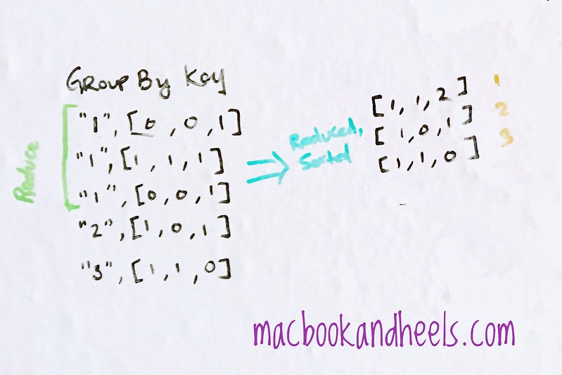
The diagram I drew above shows how the data could look like to transform the list of timestamps into a list of tuples by using a key. If we look at the data types of such a function would be [timestamps] -> [(weekNumber, weekData)] or even more abstractly, [t] -> [(w, [d])] With actual types it would be func :: UTCTime -> (Int, [Int])

There’s two parts to each tuple, and a list of tuples. To get the list of tuples, I wrote two functions to break up the workflow, to make it easier for me as a beginner to retrospectively read my code.

Let’s start with the second element, the [d] part. I wanted to create a list of element that represent a marked week, which takes the day of the week Int and returns the week [Int].

markWeek :: Int -> [Int]
markWeek dayIdx = xs ++ [norm] ++ ys
    where
        xs = replicate (dayIdx-1) 0
        ys = replicate (6-dayIdx) 0
        norm = 1 / 21             -- hardwire the max number for now

Next I worked on the first element of the tuple, which is the week number w. You can get the week number with the time-formatter formatTime.

i is defined as the week number minus 9. March weeks are weeks 9+ in the year 2017 so I subtracted 9 to get a starting index of 0 for the chart.

I decided to combine that as a where clause when returning the output of the tuples that contains the week number and list of day values using the function produceTuples.

produceTuples :: UTCTime -> (Int, [Int])
produceTuples timestamp = (w, markWeek dayIndex)
    where
        dayIndex = read (formatTime defaultTimeLocale "%u" timestamp) :: Int
        w = (read (formatTime defaultTimeLocale "%U" timestamp) :: Int) - 9

With these two functions, I could transform the list of timestamps into a list of tuples. Will let you browse the notebook to see how the output looks like. Let’s keep moving on, still some work left…

Sorting and grouping

At this point I was running out of steam and found some applicable answers on StackOverflow. It had been nearly two weeks since installing iHaskell and really wanted to have working code…!

Someone shared this sortAndGroup function on StackOverflow: How to group similar items in a list using Haskell? that takes a tuple and does some black magic to group things. One day I’ll understand the Map library…

import Data.Map
sortAndGroup assocs = toList  fromListWith (++) [(k, [v]) | (k, v) <- assocs]

Someone shared this reduction function on StackOverflow: Sum a list of lists? that combines a list of lists. A little less mysterious, as it shows most of things I’ve seen before, the map function and the sum function. reduction transposes columns to rows and sums them…

import Data.List
reduction input = Prelude.map sum . transpose  (input)

Using all that I’ve learned so far, I can produce an intermediary list of lists sample that is ready to be reduced into chartData.

Ooo, I squeezed in a nested list comprehension, fancy fancy

let sample = sortAndGroup [ getMM x | x <- march]
let chartData = [ [ 1- e | e <- reduction  snd weekly] | weekly <- sample]

To be quite honest, I’m not sure if the correct values are returned. I have not verified the output values, and mysteriously I’ve got 4 weeks in chartData, but we have the correct data type so I’m pressing onwards for now. My strategy for this code was to get something working, then edit later for precision, that way I don’t get hung up on perfecting things to the point of not finishing.

3. Setting up Plots with iHaskell

iHaskell Configs

Getting iHaskell to work with inline charts takes some extra dependencies. I edited both the ihaskell.cabal and stack.yaml files to build a working exec of jupyter working with plots

which one is right? ¯\_(ツ)_/¯ I will write a separate blog post when I figure out exactly whether it’s cabal or stack, or both that you need to use for installation. For now just know that several dependencies were added to the list, the ones that are required to work with plots:

• plots
• lens
• optparse-generic

For any further dependencies, you’ll need to add to list as well in ihaskell.cabal and/or stack.yml files and rebuild. I didn’t have time to look into a more efficient workflow yet. Hopefully such a thing exists!

For the diagram function to work (this is needed for displaying inline charts), you need to install ihaskell-display as well.

Heatmap examples

Plots version 0.1 was uploaded November 20, 2016. Right now it’s in version 0.1.0.2. There are fewer examples than Matplotlib, however Matplotlib was created in 2002, now at version 2.0.0 and has a much larger community of active users.

Of the existing heatmap plots, they are more like toy examples and have a lot of mystery surrounding their existence. It uses the diagrams library, which I’m also unfamiliar with.

All of the charts look pretty much like this, with the tick labels on the sides and the legend to the right. Not sure if it’s possible to tweak the appearance - answering that question remains to be an exercise.

Example of heatmap generated by plots

What I can do so far is show you how the code looks like for creating an inline chart in ihaskell.

Creating plots

The example code uses plain ole import Plots to get all the functions. Instead of doing that as a quick and dirty, I searched thru the documentation for the exact location of each function of each module, as a way to become more familiar with the library.

import Plots.Axis  (Axis, r2Axis)
import Plots.Axis.ColourBar (colourBar)
import Plots.Axis.Render (renderAxis)
import Plots.Axis.Scale (axisExtend, noExtend)
import Plots.Style (axisColourMap, greys)
import Plots.Types (display)
import Plots.Types.HeatMap

Furthermore, I hunted down further more types and functions that are needed to get a semblance of the example code working.

import Control.Lens ((&~), (.=))
import Diagrams.Backend.Cairo (B, Cairo)
import Diagrams.TwoD.Types (V2)
import Diagrams.Core.Types (QDiagram)
import IHaskell.Display.Juicypixels hiding (display)

So many imports to create a little chart…. this territory into dataviz with haskell is super new to me, and I’m not really sure if it’s indicative of working with Haskell libraries in general, or working with output or graphics. Could be all dimensions that makes it feel like I’m tip-toeing on the cutting edge.

For the example below, I didn’t edit much beyond the example other than changing the color from magma to greys. Figured a monochrome palette would be a simpler design than a rainbow colored one.

heatMapAxis' :: Axis Cairo V2 Double
heatMapAxis' = r2Axis &~ do
  display colourBar
  axisExtend Control.Lens..= noExtend
  axisColourMap Control.Lens..= greys
  heatMap'  reverse chartData

heatMapExample' = renderAxis heatMapAxis'

and finally to show this diagram in the notebook:

--- for the inline display

import IHaskell.Display.Diagrams
diagram heatMapExample'

And that’s it! We got a chart! It doesn’t look quite correct, probably the sortAndGroup and reduction need tweaking, however I GOT A CHART

This was my stopping point to write up a tutorial based upon my foray into uncharted territories. All the code shown in this tutorial is also available in this notebook.

final closing thoughts…

It was a good exercise to try replicating Python code in Haskell, this exercise pushed me to move beyond comfort zones in coding and challenged me to try workarounds and read the documentation carefully (and even ask others for help). Even though I want to further tweak the chart to make it perfect, at the time I want to remind myself to acknowledge that it was a huge accomplishment to have reached working code, as there’s such as small community of folks working on graphics related problems in the first place.

Acknowledgements

Many thanks to Libby in helping to find the correct documentation sections to read, and working with me through the installation and type error messages, which was helpful in overcoming some of the getting started obstacles. Also general sympathy from the others at weekend office hours regarding installation woes helped me feel better that I wasn’t alone in struggling with confusing build messages. Finally, many thanks to the nlang.nyc bloggers for tips on improving blog post writing workflow!